MAGNETOTELLURIC ANALYSIS: USE OF INVARIANCES IN MOHR CIRCLES

¹NGUYỄN THÀNH VẤN, ²LÊ VĂN ANH CƯỜNG

Department of Geophysics, University of Natural Sciences,VNU-HCM, Hồ Chí Minh City

Abstract: The magnetotelluric analysis is one of the methods used in the research on inhomogeneity of 2D and 3D electric environments, whose depths are about tens kilometers. Explaining magnetotelluric data is to get useful arbitrary parameters from a general magnetotelluric impedance tensor. Invariances are drawn from different methods to express the characteristics of 1D, 2D, and 3D models.

I. INTRODUCTION

The fundamental model of MT method is created by Tikhonov and Cagniard. In the model, MT wave transfers into a horizontally stratified earth bed, and the relation is expressed by:

; (1)

with Z: Tikhonov-Cagniard general impedance describing electrical conductivity distribution versus depth z.

(2)

where: and (3)

: Unit vectors in Cartersian axes, direction goes down.

General MT impedance Z is considered to be the relation between components and .

In the 1950s, the experiment environment in which Berdichevsky and Cagniard established impedance Z is a horizontally electrical stratified earth case.

(4)

However, because real environments are usually electric nonlayered, general impedance is considered as a tensor built from and in order to improve MT method.

Berdichevsky and Zdanov [1] said that there was an invariant relation between MT components, which expressed electrical conductivity distribution in the earth. It is an algebraic relation:

(5)

where is an arbitrary vector, which has properties of inducing field and affecting field, and are operators dependent on electrical conductivity distribution of environment and frequency. If they can be converted mutually, is a matrix to define linear relation between components of field.

II. PROPERTIES OF GENERAL IMPEDANCE TENSOR

Its property is dependent on kinds of model. 1D structure, 2D structure and 3D structure are examined in turn.

- 1D structure: Electrical conductivity distribution only varies through the depth. The model of Cagniard is 1D structure. In this model, equations Z_xx = Z_yy = 0 and Z_xy = −Z_yx = Z are always right in arbitrary measured axes.

(6)

The components Z_xy and Z_yx of general impedance tensor are related with the change of electrical property versus depth, but Z_xx and Z_yy are related with the change of electric property versus horizon.

- 2D structure: Electrical conductivity distribution varies through depth and a horizontal axis such as x-axis or y-axis. The horizontal axis, which has conductance =const, is called as the homogenous axis. Polarized electromagnetic field is divided into two parts:

1. Parallel (//) or polarized electric field (in case the electric field is polarized along homogenous axis).

2. Perpendicular () or polarized magnetic field (in case the polarized magnetic field is perpendicular to homogenous axis).

and are respectively parallel and perpendicular components of general impedance tensor. Therefore, it has zero element on the diagonal.

(7)

- 3D structure: Electrical conductivity distribution varies through depth and horizontal axes such as x-axis and y-axis. From diversity of these structures, people use symmetric cylinder structure in which general impedance tensor is simplest. Assuming that the direction of x-axis is the direction of symmetric axis, Z_r and Z_t are centripetal and tangential components of general impedance tensor. It means that the general impedance tensor has zero elements on the diagonal:

(8)

3D symmetric cylinder structure and 2D structure are same in the shape of general impedance tensor.

III. MOHR CIRCLES METHOD

The Mohr circles method, most commonly met in the analysis of mechanical stress, is used to depict magnetotelluric impedance information, taking the real and quadrature parts of magneto-telluric tensors separately.

Tensor =

Components of rotating tensor :

(9)

where

(10)

Complex A = A_r+iA_q, where A_r and A_q are, respectively, real and quadrature. Therefore, we extract circle equations for real and quadrature parts from the components of the tensor :

(11)

where

(12)

(13)

A plot of Z’_xx against Z’_xy, as the measuring axes rotate, then describes a circle, where Z’_xx and Z’_xy are the values that would be measured with axes rotated clockwise from those that gave the initial values of Z_xx and Z_xy. Similarly, the components Z’_xy and Z’_yy also form the relation through a circle equation.

Invariants with rotation of the measured axes: because Z₁ and Z₂ are invariants, the distance from the origin of axes to the circle center is invariant, which is called “central impedance” [3]. Denoting the central impedance by Z^L, its value is given by:

(14)

Other invariants are the values of the circle radii R_r and R_q.

If the circle is offset from the Z’_xy-axis, the offset can be expressed by an angle or . The value of tan is showed:

(15)

Now, we consider the relation between Mohr circles and the 1D, 2D and 3D structures.

- 1D structure: , the circle reduces to its central point, which is on the horizontal Z’_xy-axis.

- 2D structure: the circle is centered on the horizontal axis, and cut the horizontal Z’_xy-axis at two values.

- 3D structure: the circle center moves off the axis, and the invariant is different to zero. For highly anisotropic data (either 2-D or 3-D), the circumference of the circle approaches the origin of the axes (Lilley, 1993a).

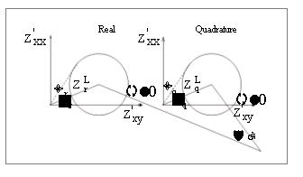
Figure 1. A pair of real and quadrature circles for a tensor, showing the set of invariant.

From inspection of the previous figure (Fig. 1), one straight-forward set can be seen to be:

1. Z^L, the distance from the origin of axes to the circle center, which gives the 1-D “scale” of a matrix, and is its 1-D kernel.

2. , an angle which gives a measure of the two dimensionality or anisotropy of a matrix, defined as:

3., an angle which gives a measure of the three dimensionality of a matrix; Z^L, , and have values for both the real and quadrature matrices of the tensor, and thus comprise six invariants.

A seventh invariant, which is a further parameter of three dimensionality, links the real and quadrature parts of a tensor and may be expressed as: ; where the angle is between the horizontal axis and the line linking the circle center to the observed point. and refer to the values of for the real and quadrature parts of a tensor, respectively.

Example: 3D impedance tensor

(a)

(b)

From the Fig. 2. the Mohr method shows the 3D structures of the environments. In Fig. 2. (b), although the quadrature Mohr circle shows 2D structure, the structure is 3D (because, in the real part, the invariant is different to zero).

IV. ASSESSMENT

Simons Spritz’s approach gives less information (6 parameters). The Eggers’s parameters are rather similar to La Torraca and Yee’s (8 parameters) but the beginning ideas to establish them are different. The principal axes of polarization ellipses of eigenvector pair (E_i, H_i) are perpendicular in Eggers’s method (the biorthogonal method). On the other hand, in the La Torraca and Yee‘s method, the principal axis directions for the and vectors are not at right angles as in the biorthogonal analysis. Because of invariant phases of eigenvalues of tensor in Eggers’s method while phases of eigenvalues of tensor in La Torraca and Yee’s method are variant (although they vary little), Eggers’s method is more effective. The Mohr circles construction (Lilley’s method) gives seven invariants of a tensor which explain the properties of 1D, 2D and 3D environment clearly and easily understandable. To research Mohr circles method further, we use it to analyze 3D model data order to draw helpful geological information.

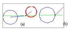
Figure 2. Real (bold line)
and quadrature (thin line) Mohr circles in the 3 D examples.

- 3-D magnetotelluric modelling: A 3-layer model whose first layer contains 3D conductivity masses is researched at frequency 2700 Hz. The 3D conductivity masses are ellipse-shaped mass and sphere mass. The ellipse-shaped mass has major axis a = 50 km, minor axis b = 12.5 km, conductivity S_c of ellipse center and conductivity S_o of the ellipse outer. The sphere mass has radius r = 5 km and conductivity of the sphere mass S_t. The distance between the center of sphere mass and the major axis of ellipse-shaped mass is 7.5 km, and the distance between the center of sphere mass and the minor axis of ellipse-shaped mass is 5 km.

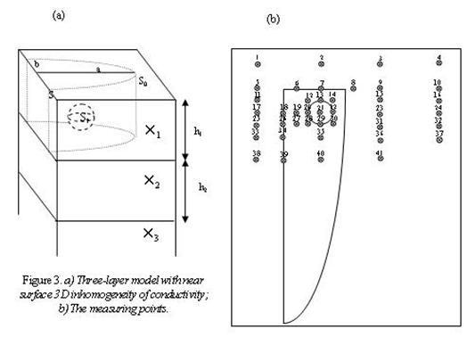
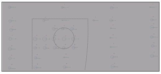
Figure. 4. Real (bold) and quadrature (thin) Mohr circles in the 3D model.

The 3D model: Resistivities of three layers are, respectively: =100; =1000000;=1;

Conductivity S_c of the ellipse center: S_c =10 CM;

Conductivity S₀ of the ellipse outer: S₀ = 10 CM;

Conductivity S_t of the sphere mass: S_t = 100 CM;

The depths of the first layer and the second layer: h₁ = 1 km; h₂ = 200 km.

1. Analysis of the 3d model:

- Mohr circles method:

At the measuring points 1-5, 7-11, 13, 15-26, 29, 31-33, 35-37, 39 and 40, the

Table 1. The set of invariant of the 3D model.

STT
1	0.000015	0.000203	18.03023	12.90871	1.859049	1.547317	2.125996
2	0.000015	0.000205	13.40122	9.593889	0.572939	0.720012	1.235592
3	0.000018	0.000271	16.13138	15.26543	0.502306	0.338899	1.079667
4	0.000013	0.000184	7.56186	4.486621	1.775164	1.290494	11.61628
5	0.000015	0.000209	19.8633	14.7104	1.162498	0.932863	0.992373
6	0.000015	0.000209	20.11097	16.15612	7.789108	6.256836	6.457061
7	0.000013	0.000183	5.066163	3.262733	2.015711	1.448568	31.09535
8	0.000015	0.000214	12.43617	10.04313	-3.56432	-3.24952	3.627354
9	0.000034	0.000516	21.54779	19.78241	-1.21088	-1.14076	0.030031
10	0.000016	0.000212	22.79522	17.28933	1.064586	0.874946	0.837864
11	0.000017	0.000229	28.482	23.23413	5.909015	4.77612	2.404132
12	0.000019	0.000265	29.36073	25.06058	9.340026	7.76614	2.746595
13	0.00002	0.000291	19.08616	16.07348	0.763432	0.495173	0.759273
14	0.000019	0.000274	23.11654	20.36288	-6.58996	-6.03368	0.752431
15	0.000021	0.000317	8.02095	6.979198	-3.84067	-3.52215	2.313074
16	0.000034	0.000508	22.26512	20.4194	-2.42938	-2.32048	0.174716
17	0.000016	0.000211	21.61166	16.49809	-0.36782	-0.1184	0.634357
18	0.000016	0.000215	28.10045	22.1313	-0.57066	-0.51298	0.060401
19	0.000017	0.000227	31.7643	26.14267	-0.75517	-0.77698	0.164174
20	0.000022	0.000306	25.92506	22.06239	-0.14975	-0.2335	0.257288
21	0.000028	0.000401	23.8888	21.41278	0.093607	0.028576	0.175762
22	0.000022	0.000317	22.00075	19.50587	-0.1715	-0.24801	0.485068
23	0.000022	0.000321	6.467167	5.682756	-1.06338	-1.00927	0.590644
24	0.000029	0.000439	15.3243	13.95562	-1.99235	-1.89829	0.109096
25	0.000035	0.000521	20.21577	18.54821	-2.22631	-2.14347	0.160561
26	0.000016	0.00021	24.91441	19.1862	-1.63166	-1.15395	1.016015
27	0.000017	0.000226	29.22115	23.64501	-7.06008	-6.02628	2.084077
28	0.000019	0.000262	27.33654	23.11352	-9.84447	-8.49831	2.557173
29	0.000021	0.000295	19.46554	16.59716	-0.8483	-0.89335	0.26702
30	0.00002	0.00028	24.92287	22.26862	5.900111	5.160111	1.135459
31	0.000021	0.000312	4.807794	4.528576	1.679112	1.480348	3.761664
32	0.000013	0.000514	43.99519	20.01832	-5.67866	-2.18032	36.65731
33	0.000015	0.000207	24.54191	19.07863	-0.64937	-0.02775	1.411758
34	0.000015	0.000205	20.42065	15.95597	-9.40079	-8.20674	4.797871
35	0.000013	0.000191	10.00696	7.048838	-3.77989	-3.97125	11.31574
36	0.000017	0.000245	21.83839	19.17688	2.25696	1.449625	3.142483
37	0.000035	0.000521	20.18581	18.5102	-3.11462	-2.99428	0.363877
38	0.000013	0.000178	16.64263	12.6226	-7.33216	-7.20092	1.191505
39	0.000014	0.000189	23.8599	18.13984	-2.361	-1.93338	1.287537
40	0.000013	0.000183	21.25694	16.7339	-2.25421	-1.8297	1.172901
41	0.000026	0.00039	21.73615	20.01137	-6.5198	-5.98825	0.047091

invariants are quite small (), radii of real and quadrature Mohr circles are nearly zeros. The centers of the Mohr circles are in the horizontal axes Z_xy. Therefore, they show 1D, 2D structures of the model environment. To explain this, we consider locations of the measuring points expressing the affect of the sphere and ellipse-shaped anomalies. The points 5, 7-10, 18, 26 and 39 are in the axis of ellipse mass. The points 17, 19-24, 2, 13, 29, 35 and 40 are in the axis of sphere mass. The points 1, 3, 4, 11, 15, 16, 25, 31-33, 36 and 37 are far from two masses.

At the measuring points 6, 12, 14, 27, 28, 30, 34, 38, and 41, the invariants change onsiderably . The centres of the Mohr circles move off the horizontal axes Z_xy and the differ from zeros. The inhomogeneity of the environment is expressed clearly. Again, locations of the measuring points express the affect of the sphere and ellipse-shaped anomalies to explain the inhomogeneity. The points 6, 27, 34, 38, and 41 sit near the boundary of two anomaly masses. Especially, the 3D points 12, 14, 28, and 30 affected by sphere mass and the 2D points 13, 20, 22 and 29 create boundary of two anomaly masses ( in the Tab. 1, the bold and italic rows are used for the points 12, 14, 28 and 40; the bold rows are used for the points 13, 20, 22 and 29.).

When the biorthogonal method is applied to analyze the 3D model data, the result also makes the sphere mass outstanding. In the measuring points 12, 14, 28 and 30, the directions of the red bold are directed toward the sphere mass. In the measuring points 13, 20, 22, and 29, the linear polarized ellipses show 1D and 2D structures of the model. Therefore, the measuring points 12, 14, 28, 30, 13, 20, 22, and 29 create a boundary of two anomaly masses (Fig. 5.).

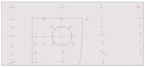
Figure 5. E-polarization ellipses for both eigenstates in the 3D model.
E₁(red bold line); E₂(blue line).

V. CONCLUSION

By considering two real and quadrature elements, the Mohr circles method gives the useful approach to analyze the magnetotelluric data. With information gotten from the set of seven Mohr circle parameters, we have enough evidences to affirm an 1D, 2D and 3D environment, then, continue to measure or choose data to establish a reserve model problem.

REFERENCES

1. Berdichevsky M.N., Dmitriev V.I., 1992. Magnetotelluric sounding of horizontally homogeneous media. Moscow (in Russian).

2. Berdichevsky M.N., Nguyen Thanh Van., 1991. Magnetovariational vector. Izv. Akad. Nauk USSR, Fizika Zemli, 3 : 52-62. Moscow.

3. Lilley F.E.M., 1998. Magnetotelluric tensor decomposition: Part I. Theory for a basic procedure. Geophysics, 63 : 1885 -1897. Part II. Examples of a basic procedure. Geophysics, 63 : 1898-1907.

4. Nguyễn Thành Vấn, 1996. The methods of assessment and classification of the geoelectrical inhomogeneities in magnetotelluric data processing. J. of Sci. and Techn., 4 : 48-52. Hà Nội (in Vietnamese).

5. Nguyễn Thành Vấn, 2005. Magnetotelluric tensor: Decomposition and applications. Sci. and Techn. Dev. 8/8 : 26-34. VN Nat. Univ.-HCM City.

6. Nguyễn Thành Vấn, Lê Vân Anh Cường, 2008. Magnetotelluric analysis: Mohr circles. Sci. and Techn. Dev., 11/11 : 5-11. VN Nat. Univ.-HCM City.