APPLICATION OF ELECTRICAL RESISTIVITY AND HYDROGEOLOGY
MODELLING METHODS TO MAP
AND FORECAST THE SALTWATER INTRUSION IN THÁI BÌNH
PROVINCE
1NGUYỄN NHƯ TRUNG, 1TRỊ
NH HOÀI THU, 2NGUYỄN VĂN NGHĨA
1Institute of Marine
Geology and Geophysics, VAST;
2Division
of Water Resource Management, MNRE
Abstract: This paper focuses on the application of
electrical resistivity and hydrogeology modelling to map the
freshwater/saltwater interface and forecast the saltwater intrusion caused by
the freshwater withdraw. Based on VES data and pore water conductivity,
measurements were carried out in Thái Bình coastal plain from 2006 to 2007, the
total dissolved solids (TDS) and the spatial distribution of saltwater /
freshwater interface in the Pleistocene aquifer were predicted and mapped. Significant changes in pore water
conductivity from the north to the south were detected by these methods. A low
resistivity value of the Pleistocene aquifer (< 9 ohm) or high conductivity
of Pleistocene pore water (> 0.24 S/m) implies the saltwater / freshwater
boundary. The results of spatial distribution of TDS indicate the saltwater
affected aquifer is confined to the southern part of the Thái Bình province
(from the longitude 20030’ N to the south).
Based on the modified Archie’s law and the
correlation between the conductivity and TDS of the pore water suggested by the
authors, two empirical relations between pore water resistivity of the
Pleistocene beds and bulk resistivity and pore water resistivity and TDS are
obtained. They can be used to convert the computed bulk resistivity and pore
water conductivity to the TDS, and thus, leading to the confine of the
groundwater contamination. Based on the TDS maps, the hydrological modelling
method is conducted for forecasting a safety-pumping rate of the region and
groundwater contamination from present time to the 2030 year.
I. INTRODUCTION
Thái
Bình, a coastal plain province, is fast urbanized and becomes an agricultural
and industrial centre in the Red River Delta. With the complicated hydrogeological
conditions, although having abundant reserves of groundwater, but almost
aquifers are confronted with saltwater intrusion.
Although there is not a large-scale groundwater exploiting station, but
thousands of UNICEF wells had been drilled uncontrollably to meet the
freshwater demand, reducing the water table. It may be the main reason of
saltwater intrusion. Actual state, rate, forecasting and protection of
saltwater intrusion should be considered to exploit the groundwater resources
substantively. The conventional method is used to investigate
saltwater intrusion is chemical analysis of water sample. This method gives
very highly precise results. However, it consumes many time and intensive and
expensive labour. Another method has been widely and effectively used to
investigate the saltwater intrusion is the electrical resistivity method [3, 4,
10-15]. Based on measuring apparent resistivity of the aquifer on the surface,
the method allows us to determine saltwater/freshwater interface from the resistivity
changes of the aquifer. Main advantages of the method are fast, cheap and
reliable results.
In
this paper, both the electrical resistivity and chemical analysis have been
conducted in this study for investigating the saltwater intrusion in Pleistocene
aquifer in Thái Bình Province.
The aquifer structures and their bulk resistivity are determined by the
inversion of the VES data. The pore-water conductivity and its TDS of selected
samples are measured and analyzed in the field and in laboratory. The
distribution of the TDS of the region is mapped for the 2006-2007 years.
Finally, the distribution of saltwater intrusion is also forecasted for the
2015, 2020 and 2030 years by the hydro-geological modelling method.
II. GEOLOGICAL SETTING
The
study area is located between the longitudes 106006’33” and 106037’35”
E and the latitudes 20005’15” and 20043’57”N. It is about
1542 km2 large and consists of 8 districts and 1 city. The
topography of the study area is quite flat. The average elevation is 1-2.5 m
above the sea level. The Quaternary alluvial sediments, including mud clay,
stiff clay, silty-clay, silt-loam, sand, and gravel cover it completely. The
Quaternary sediments may be divided into 5 formations [6]: Lệ Chi Fm (QI lc),
Hà Nội Fm (QII-III hn), Vĩnh Phúc Fm (QIII2 vp),
Hải Hưng Fm (QIV1-2 hh), and Thái Bình Fm (QIV3
tb). There is unconformity separating Quaternary sediments and
Paleozoic-Neogene sandstone, siltstone and limestone. There are three aquifers
in Quaternary sediments namely: Upper Holocene aquifer (qh2), Lower Holocene aquifer
(qh1), Pleistocene aquifer (qp) and unconfining Quaternary layers
namely: Hải Hưng Upper Sub-Fm (QIV1-2 hh2)
and Vĩnh Phúc Upper Sub-Fm (QIII2 vp2). According to the
hydrogeological data, the main aquifer in Quaternary sediments are Pleistocene
one. It is considered to be at the depth of 26-143 m and its average thickness
is about 29-127 m. The water qualities of Pleistocene aquifer can be clearly
divided into 2 parts: the salt water (TDS >1 g/l) in the southern part and
the fresh water (TDS <1 g/l) in the northern part of the province.
III. MEASUREMENT AND INTERPRETATION METHODS
1. Electrical resistivity method
Vertical
electrical sounding (VES) has been used for estimating the geoelectrical params
of the structure and TDS of aquifer in the periods 1996 and 2006-2007. To
determine the geoelectrical structure, 210 VES stations measured in 1996 and 79
VES stations measured at pumping wells in 2006-2007 were used [8]. Apart from
VES data, 222 pore water samples at the pumping wells were collected for
measuring electrical conductivity and analyzing chemistry [8].
a. Geoelectrical structure of Quaternary sediments:
The
VES data are interpreted by the forward-inversion methods, which constrain by
the available well data. The bulk resistivity and thickness of layers at each
VES station are gotten from this interpretation process. The structure of
geoelectrical cross-section in the study area is determined by the combination
of the interpretation results. It consists of 5 layers in Quaternary sediments
corresponding to the 3 aquifers and 2 unconfined layers as mentioned above:
- First layer: lying on the top of
geological cross-section. Its average thickness is
about 9 m and resistivity value is in range of 8-70 Ωm.
- Second layer: average
thickness - 18 m, resistivity value - 0.7-50 Ωm.
- Third layer: average
thickness - 17 m and resistivity value - 3.2-16 Ωm.
- Fourth layer: average
thickness - 18 m and resistivity value - 5.3-30 Ωm.
- Fifth layer: average
thickness - 41 m and resistivity value - 2.2-14.3 Ωm.
- Sixth layer: average
depth - 110 m and resistivity value - 5-60 Ωm.
As
mentioned above, the main aquifer in Quaternary sediments is Pleistocene one
(qp), so in this study we only investigate the saltwater intrusion in this
aquifer.
b. Formation factor of Pleistocene aquifer: As you may know, the
relationship between the bulk resistivity and pore water resistivity of the
aquifer is presented by the modified Archie’s law: rbuk = Frw; where F is the formation factor of aquifer; rbuk is the bulk resistivity
of aquifer and rw - pore water resistivity [2].
According
to Archie’s law, each aquifer is characterized by one formation factor. The
change of bulk resistivity depends on the change of pore water resistivity [2].
Basing on the bulk resistivity of the qp (rbuk) and pore water
resistivity (rw) at 25 pumping wells, we have a relationship
between bulk resistivity and pore water resistivity as illustrated in Fig. 1.
The regress formula can be obtained as:
rbuk = 2.20 rw (1)
The
formation factor of the qp is determined as: F = 2.2. Substituting the bulk
resistivity for the equation (1), we can determine the pore water resistivity
of the qp.
c. Determining TDS and chloride from pore water
resistivity: The analytical result of TDS and content of chloride, bulk resistivity
and pore water resistivity at 25 pumping wells are illustrated in the Fig. 2.
Based on these distributions, the following regress equations can be
obtained:
Y = 4099.52*X (2)
Where
Y is TDS in water (mg/l); X - pore water resistivity (S/m);
And Y = 2317.30* X-64.67
(3)
where
Y is content of chloride (mg/l), X - pore water resistivity (S/m).
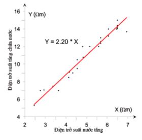
Figure 1. Correlation
between bulk and pore water resistivity of the qp.
The empirical formulas (1), (2) and (3) allow us to calculate the TDS
and content of chloride of qp from pore water resistivity or bulk resistivity.
2. Hydrogeological modelling method
Based on the aquifer structures and their
distribution of TDS of aquifer, the forecasting
problem of saltwater intrusion is developed from the solution of two following
problems [1, 5, 7, 9]:
-
Flow modelling problem, the argument is a distribution of water table in space;
-
Transmitted material problem, the argument is a distribution of TDS in space.
So far, these two
problems are solved fairly good by finite-difference and finite-element
methods. Many hydrogeological laboratories in the world have been developing
these problems into a package software to compute three-D groundwater flow and
contaminant transport simulations. In this paper, the authors used the Visual
Modflows software of Watertoo Company, Canada [9] for our calculations.
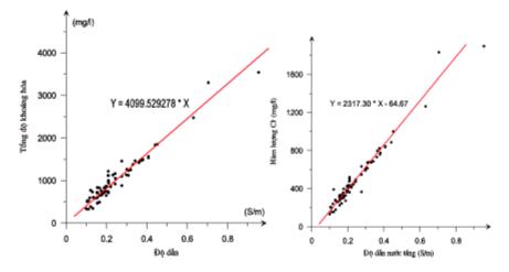
Figure 2. Relation between (a) TDS and pore
water resistivity
and (b) content of chloride and pore water resistivity.
The general calculating
steps are performed as follows:
- Assigning boundary condition: In the
east side along the Bắc Bộ (Tonkin) Gulf, the boundary condition is imitated
the first class and the water table is constant and equals H = 0 m, total
solute chemitry in seatwer is 3,0 g/l. The river systems are imitated third
class boundary condition and assume that they are not under the influence of
saltwater intrusion.
- Assigning the aquifer and aquitard:
All structural data of aquifer and aquitard and the TDS of Pleistocene are used
for the above interpretated results. All other properties and relevant params,
such as permeability, storage coefficients, discharge and recharge rate ..., of
the aquifer and aquitard are referred from hydrogeological reports [6].
- Adjusting the parameters of the model:
All params of the model, for example, permeability, storage coefficients,
discharge and recharge rate ..., will be adjusted by the stable inversion and
unstable inversion problems. Apart from adjusting, the hydrogeology param, the
TDS in 2006-2007, the statistic actual pumping rate are also used for adjusting
the material spreading params. The TDS in 2006-2007 is used as solution
constrained condition during performing the inverse procedure. Fig. 3 is the
TDS measured in 2006-2007 (Fig. 3a) and the TDS for the year 2006 is
calculated from the adjusted input
params (Fig. 3b). The measured TDS and calculated TDS are similar to the same
show that the adjusted params for the modelling can be accepted.
III. SALTWATER INTRUSION BOUNDARY AND
FORECASTING RESERVES
1. Saltwater intrusion boundary in the Pleistocene
aquifer (qp)
The
above measurement and interpretation data allow us to map the spatial
distribution of chloride and TDS of the qp in
2006-2007 (Fig. 4). The Fig. 5a shows the content of chloride changing
from 0.2 g/l in the north to 12.5 g/l in the south.
Most northern part of study area the content of chloride is less than 0.5 g/l
(account for 40 % area). In the southern part, the content of chloride is very
high, changing from 0.5 to 12.5 g/l.
In the Fig. 4b, the spatial distribution of TDS is the same as that of
chloride. the TDS also increases from the north to the south of the study area.
The highest TDS is 21 g/l located in the southern part. If we take the 1 g/l
TDS contour is the boundary of the salt/fresh water (the red line in Fig. 4), all
fresh-water area is distributed in the north of the study area and accounts for
about 605 km2.
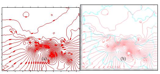
Figure
3. Model of params adjusted by inversion problem based on TDS measured
in 2006-2007: (a) TDS measured in
2006-2007; (b) TDS calculated for 2006
from the adjusted params of the model.
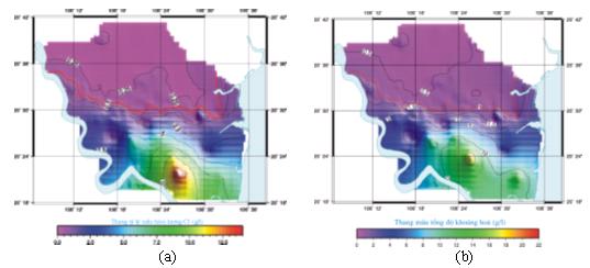
Figure 4. Spatial distribution of content of
chloride (a) and TDS in 2006-2007
(b) in Thái Bình Province.
2. Estimating the fresh-water exploited
reserves of Pleistocene aquifer
To estimate the exploited reserves of the freshwater area, we set up
every 2 km a pumping well for all freshwater area (see Fig. 5a). We will have
215 pumping wells and total pumping rate is 118250 m3/day (550 m3/day
per well). The calculated results of the reduction of water table and saltwater
intrusion for the year 2010, 2015, 2020 and 2030 are as follows:
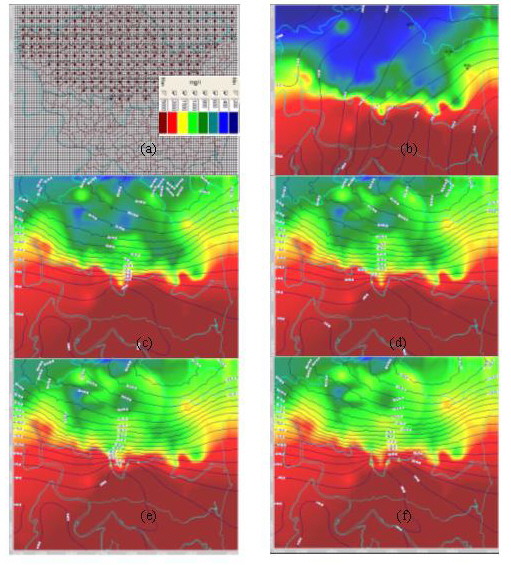
Figure 5. Water level and TDS
of the Pleistocene aquifer calculated for the 2006 (b), 2010 (c), 2015 (d);
2020 (e) and 2030 (f) years.
The water level in the qh2 and qh1 aquifers change
in the range of -1 to 4 m. Since 2015, the eastern part of Hưng Hà District the qh2 and qh1
aquifers is being to take shape the drawdown funnel having water level of 0,5 m
in 2020 and -1 m in 2030. The salt/fresh water boundary of the qh2
aquifer changes lightly by time. The TDS varies from 2-3 g/l in the saltwater
area and reduces in the freshwater area. The evidence for that is the
occurrence of the freshwater spots in the qh2 aquifers.
The qh1 aquifer has saltwater intrusion completely at 2006
with the TDS of 2-3 g/l. By the time, the water exploiting activities making
the freshwater penetrated into qh1 from qh2 desalts the
northern part of the region. The freshwater area in this aquifer is spreading
by the time.
The
forecasting results of the water level reduction and saltwater intrusion of the
qp are shown in Fig. 5b, 5c, 5d, 5e, and 6f. The lowest elevation of the
forecasted water levels is -8 m in 2010, -12 m in 2015, -14 m in 2020 and -16 m
in 2030. The water flow direction is moving from the south to the north. The
centre of the drawdown funnel is located in the centre of the Thái Thụy
District. The salt/freshwater boundary moves up strongest to the north
direction. The Thái Thụy District is salted completely in the year 2030. The
salt/freshwater boundary is spreading to the center of Đông Hưng, Hưng Hà and
Quỳnh Phụ districts. The calculated results also show that the horizontal salt
rate is predominated. The evidence for that no isolated saltwater zone is
occurred in the freshwater area.
The
forecasted exploiting reserves are determined by the way of accounting at each
time there are how many wells still lie on the freshwater area. The result of
the exploiting reserves of the Pleistocene aquifer is as follows:
- 2006 year: total freshwater exploiting wells are 215 and total pumping rate is
11825 m3/day.
- 2010 year: total freshwater exploiting wells are 194 and total pumping rate is
106700 m3/day.
- 2020 year: total freshwater exploiting wells are 175 and total pumping rate is
96250 m3/day.
- 2030 year: total freshwater exploiting wells are 98 and total pumping rate is
53900 m3/day.
3. Estimating the
substainable pumping rate
The substainable pumping
rate is how volume of water exploited so that the salt/freshwater boundary has
no change by the time. Assuming the pumping wells are located in the centre of
every commune of the freshwater area of the qp. The pumping rate at earch well
is adjusted and operations repeated until a total acceptable pumping rate
doesn’t make change of the salt/freshwater boundary. After many interactive
computing, we have determined the substainable pumping rate for the qp is 27557
m3/day. With the pumping rate of 27557 m3/day, the
salt/freshwater boundary of the qp has no change for the 2030 year.
CONCLUSIONS
1.
The interpretation results allow us to reconstruct the spatial distribution of
the TDS, content of chloride and salt/freshwater boundary of the Pleistocene
aquifer in Thái Bình Province
for the year 2006-2007. The freshwater area of the Pleistocene aquifer account
for 605 km2, distributed mainly in the northern part of the province
including the Hưng Hà, Đông Hưng, Quỳnh Phụ and Thái Thụy districts. The TDS maps and the structure of aquifer and confines are useful data
resources for applying numerical hydrogeology modelling to forecast the
saltwater intrusion and suitable pumping rate in the study area.
2.
According to the modelling calculation, if we maintain the pumping rate of
118,250 m3/day, the freshwater reserves of the Pleistocene aquifer
may remain only about 80 %, equivalent to the pumping rate of 96250 m3/day
for the year 2020 and about 45 %, equivalent to pumping rate of 53900 m3/day
for the year 2030. To remain the current salt/freshwater boundary of the
Pleistocene aquifer, the pumping rate of the Pleistocene aquifer should be
27557 m3/day and the well net is distributed evenly in local
communes.
REFERENCES
1. Anderson
M.P., W.W. Woesseer, 1992. Applied groundwater modelling. Acad.
Press, Inc., New York.
2. Archie G.E., 1944. The
electrical resistivity log as an aid in determining some reservoir
characteristics. Am. Inst. Min. Metallurg Petr. Eng. Tech. Paper, 1422 pp..
3. Ardau F.,
Barbiere G., 1994. Evolution of phenomena of salt
water intrusion in the coastal plain of Muravera (southeastern Sardinia): 13th saltwater intrusion Mtg. Exp.
abstr., 305-312.
4. Chieh-Hou Y.,
Lun-Tao Tong, Ching-Feng Huang, 1999. Combined
application of DC and TEM to sea-water intrusion mapping. Geophysics, 64/2 :
417-427.
5. Herbert F.W., W.W. Woesseer, 1982.
Introduction to groundwater modelling. Acad. Press Inc., New York.
6. Lại Đức Hùng (Ed.), 1996. Final
report on drawing hydrogeological map, scale 1:50.000. Arch. of Dept of
Geology, pp. 105.
7. Mary P.A., W.W. Woesseer, 1992.
Applied groundwater modelling. Acad. Press Inc., New York.
8. Nguyễn Như Trung (Ed.), 2007.
Evaluating the actual state and forecasting the saltwater intrusion of
groundwater aquifer of Thái Bình coastal plain. Final report. VN Acad. of
Sci. and Techn., 150 pp.
9. Nilson G., Thomas F., 2004. Visual
mudflow guideline, Version 4.0. Waterflow Hydrogeology Software, Toronto.
10. Paul M.B., 2003. Groundwater in freshwater-saltwater environments
of the Atlantics coast. Circular 1262, US Geol. Surv., 113 pp..
11. Roberto B., E. Gavaudo,
Fr. Ardau, G. Ghiglieri, 2003. Geophysical approach to the
environmental study of the coastal plain. Geophysics, 68/5 : 1446-1459.
12. van Overmeeren, 1989.
Aquifer boundaries explored by geoelectrical measure-ments in the coastal plain
of Yemen: Case of equivalence. Geophysics, 54 : 38-48.
13. Waheidi M.M., F.
Merlanti, M. Pavan, 1992. Geoelectrical resistivity
survey of the central part of Azraq basin (Jordan) for identifying
saltwater/freshwater interface. J. of Applied Geoph..
14. Wang H.F., W.W. Woesseer, 1982.
Introduction to groundwater modelling. Acad. Press Inc., New York.
15. Zhdanov
M., Keller G., 1994. The geoelectrical methods in geophysical
exploration. Methods in geoch. and geoph., 31, Elsevier, Amsterdam-London-New York - Tokyo, 873 pp..